How to use Python linear regression method
This article mainly explains "how to use Python linear regression method". The explanation content in this article is simple and clear, easy to learn and understand. Please follow the idea of Xiaobian slowly and deeply to study and learn "how to use Python linear regression method" together!
In terms of conventional notation, linear regression parameters consist primarily of slope and intercept, where W represents slope and b represents intercept. A capital W means this is a vector. Generally speaking, it is the number of n_feauter_num, that is, how many features there are, the shape of W is (n_feauter_num,1), intercept b is a constant, and the target Y value is calculated by the formula Y=W*X+b. Generally speaking, in machine learning, the original value is Y, and the predicted value is Y_hat. Let's talk about the specific implementation steps
configuration data
construct loss function(cos function)
Calculate the gradient for W and b separately (also derive the cost function for W and b separately)
Calculate Y_hat
Multiple iterations of gradient calculation, direct convergence or iteration termination
The following gives the specific python code implementation, this code is a general code, you can arbitrarily extend W, the code to calculate loss and gradient of the vector implementation, so increase the dimension of W without modifying the code
import matplotlib.pyplot as pltimport numpy as npdef f(X): w = np.array([1, 3, 2]) b = 10 return np.dot(X, w.T) + bdef cost(X, Y, w, b): m = X.shape[0] Z = np.dot(X, w) + b Y_hat = Z.reshape(m, 1) cost = np.sum(np.square(Y_hat - Y)) / (2 * m) return costdef gradient_descent(X, Y, W, b, learning_rate): m = X.shape[0] W = W - learning_rate * (1 / m) * X.T.dot((np.dot(X, W) + b - Y)) b = b - learning_rate * (1 / m) * np.sum(np.dot(X, W) + b - Y) return W, bdef main(): # sample number m = 5 # feature number n = 3 total = m * n # construct data X = np.random.rand(total).reshape(m, n) Y = f(X).reshape(m, 1)# iris = datasets.load_iris()# X, Y = iris.data, iris.target.reshape(150, 1)# X = X[Y[:, 0] < 2]# Y = Y[Y[:, 0] < 2]# m = X.shape[0]# n = X.shape[1] # define parameter W = np.ones((n, 1), dtype=float).reshape(n, 1) b = 0.0 # def forward pass++ learning_rate = 0.1 iter_num = 10000 i = 0 J = [] while i < iter_num: i = i + 1 W, b = gradient_descent(X, Y, W, b, learning_rate) j = cost(X, Y, W, b) J.append(j) print(W, b) print(j) plt.plot(J) plt.show()if __name__ == '__main__': main()
As you can see, the resulting output is very close to the preset parameters [1, 3, 2] and 10
So easy.
step: 4998 loss: 3.46349593719e-07[[ 1.00286704] [ 3.00463459] [ 2.00173473]] 9.99528287088step: 4999 loss: 3.45443124835e-07[[ 1.00286329] [ 3.00462853] [ 2.00173246]] 9.99528904819step: 5000 loss: 3.44539028368e-07 Thank you for reading, the above is "how to use Python linear regression method" content, after the study of this article, I believe everyone on how to use Python linear regression method This problem has a deeper understanding, the specific use of the situation also needs to be verified by practice. Here is, Xiaobian will push more articles related to knowledge points for everyone, welcome to pay attention!